Fixed Depth vs Equivalent Soil Mass: Why Soil Carbon Stocks Need a Common Reference Mass
soil carbon
soil measurement
soil data
Comparing soil carbon stocks to a fixed depth can create apparent gains or losses that are really changes in bulk density. Here is how the equivalent soil mass approach fixes that, with R code to calculate it.
Soil carbon stocks have traditionally been reported to a fixed depth: Mg of carbon per hectare in the top 30 cm, for example. It seems like the obvious way to compare two sampling times, or two management practices. But a fixed depth doesn’t contain a fixed amount of soil. If bulk density changes between sampling events, the same 30 cm holds a different mass of soil, and comparing stocks at a fixed depth mixes a change in carbon with a change in bulk density.
That’s why the equivalent soil mass (ESM) approach has become the recommended standard for measuring soil carbon change (von Haden et al. 2020), and why carbon protocols such as Verra’s VM0042 require it. This article explains the concept, then works through an example using real Saskatchewan data from the Prairie Soil Carbon Balance (PSCB) report, with R code to calculate ESM stocks.
Why fixed depth can mislead
A soil carbon stock to a given depth is the product of three things:
The bulk density term is the potentially confounding factor. Management can change bulk density along with SOC. Tillage activities, compaction from equipment traffic, and changes in organic matter all can shift bulk density.
For example, a field can see an increase in bulk density due to repeat equipment traffic over time. Sampling to 30 cm before and after compaction captures more soil mass the second time, because the same depth is denser. Even if carbon concentrations barely changed, the fixed-depth stock goes up, simply because there is more soil in the sample. The reverse happens when bulk density decreases, for example as soil gains organic matter: a fixed-depth comparison can understate a real gain, or even show a loss that is really a drop in bulk density.
The equivalent soil mass approach removes this effect by comparing carbon in the same mass of soil at each sampling time, rather than the same depth.
A worked example with Prairie farm data
The Prairie Soil Carbon Balance (PSCB) project has monitored soil carbon on commercial farm fields across Saskatchewan since 1996, after the fields converted to direct seeding (McConkey 2019). Each benchmark was sampled to 40 cm in 10 cm increments, with bulk density measured at every sampling. The project’s 2019 report gives the network-average bulk density and organic carbon concentration by layer for the 88 fields sampled in both 1996 and 2018 (Table 4 of the report).
Those averages make a useful example. Between 1996 and 2018, bulk density increased significantly at every depth.
Soil mass for each layer is bulk density times thickness, converted to Mg per hectare. The SOC stock is the SOC fraction times that mass.
Fixed-depth stocks
Summing the layers to 30 cm gives the fixed-depth stock in each year:
top30 <- profiles[profiles$bottom <=30, ]fixed <-aggregate(cbind(mass, soc_stock) ~ time, data = top30, FUN = sum)fixed
  time mass soc_stock
1 1996 4090  61.15170
2 2018 4425  66.35777
On a fixed-depth basis, the 0 to 30 cm stock rises from 61.2 to 66.4 Mg C/ha, an apparent gain of about 5.2 Mg C/ha. But the soil mass in the top 30 cm also rose, from 4,090 to 4,425 Mg/ha. About 8% more soil is in the same 30 cm.
Equivalent soil mass stocks
The ESM approach picks a reference soil mass and calculates the carbon in that mass at each time. Here the reference is the 1996 soil mass to 30 cm: 4,090 Mg/ha.
To find the carbon in the first 4,090 Mg/ha of soil in 2018, we build the cumulative relationship between soil mass and carbon through the profile, then interpolate it at the reference mass using a monotone cubic spline, following Wendt and Hauser (2013) and von Haden et al. (2020). Because the profile was sampled to 40 cm, the reference mass falls within the sampled soil in both years. Extrapolating to reference mass values outside the sample range should be avoided, as that increases the uncertainty of the results.
esm_stock <-function(mass, soc_stock, ref_mass, method =c("spline", "linear")) { method <-match.arg(method) cum_mass <-c(0, cumsum(mass)) # cumulative soil mass from the surface cum_soc <-c(0, cumsum(soc_stock)) # cumulative SOC from the surfaceif (ref_mass >max(cum_mass)) {stop("Reference mass exceeds the sampled soil mass: sample deeper.") }if (method =="spline") {# monotone cubic spline: cumulative SOC can only increase with soil masssplinefun(cum_mass, cum_soc, method ="hyman")(ref_mass) } else {# linear interpolation, equivalent to Ellert and Bettany (1995)approx(cum_mass, cum_soc, xout = ref_mass)$y }}ref_mass <-sum(top30$mass[top30$time =="1996"]) # 4,090 Mg/haesm <-sapply(split(profiles, profiles$time), function(p) {c(esm_spline =esm_stock(p$mass, p$soc_stock, ref_mass, "spline"),esm_linear =esm_stock(p$mass, p$soc_stock, ref_mass, "linear"))})results <-data.frame(year =colnames(esm),fixed_depth = fixed$soc_stock[match(colnames(esm), fixed$time)],esm_spline = esm["esm_spline", ],esm_linear = esm["esm_linear", ],row.names =NULL)knitr::kable(results, digits =1,col.names =c("Year", "Fixed depth (0-30 cm)", "ESM (spline)", "ESM (linear)"))
Year
Fixed depth (0-30 cm)
ESM (spline)
ESM (linear)
1996
61.2
61.2
61.2
2018
66.4
63.0
62.9
# Change in each estimate, and the ESM change using the average mass as referencechg_fixed <-diff(fixed$soc_stock[match(c("1996", "2018"), fixed$time)])chg_spline <- esm["esm_spline", "2018"] - esm["esm_spline", "1996"]chg_linear <- esm["esm_linear", "2018"] - esm["esm_linear", "1996"]ref_avg <-mean(tapply(top30$mass, top30$time, sum))esm_avg <-sapply(split(profiles, profiles$time),function(p) esm_stock(p$mass, p$soc_stock, ref_avg))chg_avg <- esm_avg["2018"] - esm_avg["1996"]
On an equivalent mass basis, the 2018 stock is about 63 Mg C/ha, so the change is about 1.8 Mg C/ha, compared with the 5.2 Mg C/ha a fixed-depth comparison suggests. Linear interpolation gives a similar change of 1.7 Mg C/ha. The difference is the carbon in the extra 335 Mg/ha of soil that the denser 2018 soil packs into the top 30 cm.
The choice of reference mass matters. Using the average of the 1996 and 2018 masses, as the PSCB report did, gives a change of about 1.9 Mg C/ha. The report’s own ESM analysis, calculated site by site rather than from network averages, found a gain of 2.41 Mg C/ha for 0 to 30 cm (its Table 5). All of these are far below the fixed-depth estimate.
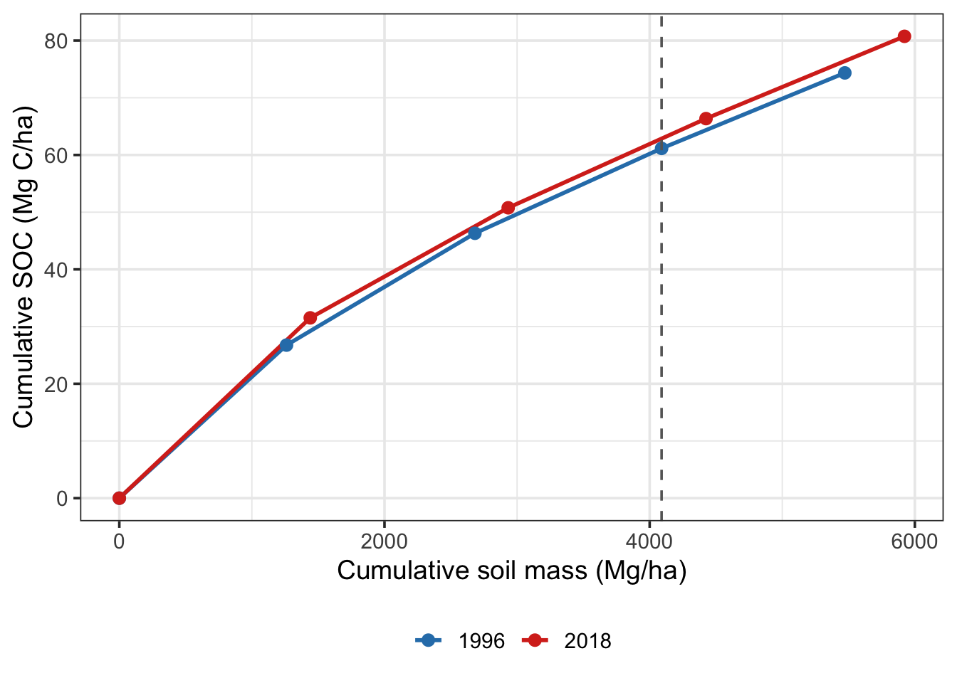
The plot shows what the calculation is doing. Each line is cumulative carbon against cumulative soil mass down the profile. The fixed-depth comparison reads each line at 30 cm, where the two years hold different amounts of soil. The ESM comparison reads both lines at the same soil mass.
Cumulative SOC against cumulative soil mass for the PSCB network averages in 1996 and 2018. The dashed line marks the reference soil mass (the 1996 mass to 30 cm). Points mark the 10 cm layer boundaries.
One caveat applies to this example: multiplying average bulk density by average carbon concentration isn’t exactly the same as averaging each field’s stock, which is one reason these numbers differ from the report’s site-by-site results. The report’s SOC stock gains, calculated site by site, are more accurate. The data in this post are just to illustrate the calculations and how they affect the results.
Linear or spline interpolation?
The function above uses a cubic spline by default, with linear interpolation available for comparison. The two methods make different assumptions about how carbon is distributed within each sampled layer.
Linear interpolation assumes carbon relationship with depth is strictly linear. It gives the same answer as the classic correction of Ellert and Bettany (1995), which removes the excess soil mass from the deepest layer at that layer’s carbon concentration. It’s simple and transparent.
Cubic spline interpolation, used by Wendt and Hauser (2013), fits a smooth curve through the cumulative points. It better reflects the way carbon concentration usually declines with depth, which matters more when layers are thick or when you report several mass-based layers. The hyman method in R keeps the curve from decreasing, since cumulative carbon can only increase with depth. This is the same approach used in the ESM R script published by von Haden et al. (2020).
With thin layers, like the 10 cm increments here, the two usually give similar results, as the two ESM columns in the table above show. With thick layers, or when the reference mass falls well inside a layer, the choice matters more.
Applying ESM to real data
Key points to consider when doing ESM calculations:
Measure bulk density every time you sample. ESM depends on the soil mass in each layer, so bulk density has to be measured at each sampling, for each layer. Assuming a fixed bulk density brings back the problem ESM is meant to solve.
Sample deeper than your target depth. If soil becomes less dense between samplings, the mass to 30 cm can fall below the reference mass, and there is no data to interpolate into. Sampling one extra layer below the reporting depth means the reference mass is always within the sampled profile. The function above stops with an error rather than extrapolating.
Choose the reference mass deliberately and report it. Common choices are the baseline mass, the mean mass across all samples, or the lowest mass observed. Using the lowest mass guarantees every sample reaches it. Whatever you choose, use the same reference mass for every comparison.
Use several sampled layers. Reporting carbon in more than one mass-based layer (for example, the masses equivalent to 0 to 15 cm and 15 to 30 cm) shows where in the profile the change occurred, which matters because practices like no-till concentrate carbon near the surface.
Account for coarse fragments and inorganic carbon. Bulk density and soil mass should be for the <2 mm fraction, and on calcareous soils the carbon should be organic carbon, not total carbon.
To apply the function to a full dataset, run it for every site and sampling time. The example below uses a small test dataset with three sites, each sampled at baseline and remeasurement in four 10 cm layers to 40 cm. Site A becomes denser, site B changes little, and site C becomes less dense, so its remeasured soil mass to 30 cm falls below the reference mass. Because every profile was sampled to 40 cm, the reference mass still falls within the sampled soil.
At site A, where the soil became denser, the fixed-depth comparison overstates the gain. At site C, where it became less dense, the fixed-depth comparison understates it. At site B, with little change in bulk density, the two methods are closer. Note that the reference mass and the fixed-depth stock both use only the layers to the reporting depth, even though the profiles were sampled deeper.
Further resources
For a more complete implementation, von Haden, Yang, and DeLucia published an R script alongside their 2020 paper: the ESM R script from the Center for Advanced Bioenergy and Bioproducts Innovation (CABBI). It handles many cores and replicates at once, calculates stocks at several reference depths, and outputs both fixed-depth and ESM results.
The takeaway
A fixed depth is not a fixed amount of soil. When management changes bulk density, fixed-depth comparisons confuse changes in soil bulk density with changes in soil carbon, and can overstate or understate the change considerably. Comparing stocks on an equivalent soil mass basis removes that bias, and it takes only a few lines of code once bulk density is measured at each sampling.
The ESM approach trades a reference depth for a reference mass. With fixed depth, the mass of soil compared varies; with ESM, the depth compared varies. That changes how the results need to be interpreted, and while ESM is not quite as intuitive as fixed depth, it minimizes the influence of varying bulk density values for carbon change over time assessments.
References
Ellert, B.H., and Bettany, J.R. 1995. Calculation of organic matter and nutrients stored in soils under contrasting management regimes. Canadian Journal of Soil Science, 75(4): 529–538. https://doi.org/10.4141/cjss95-075
McConkey, B. 2019. Prairie Soil Carbon Balance Project: Monitoring SOC Change Across Saskatchewan Farms from 1996 to 2018. Phase 1 Report. Saskatchewan Soil Conservation Association. PDF
von Haden, A.C., Yang, W.H., and DeLucia, E.H. 2020. Soils’ dirty little secret: Depth-based comparisons can be inadequate for quantifying changes in soil organic carbon and other mineral soil properties. Global Change Biology, 26(7): 3759–3770. https://doi.org/10.1111/gcb.15124
Wendt, J.W., and Hauser, S. 2013. An equivalent soil mass procedure for monitoring soil organic carbon in multiple soil layers. European Journal of Soil Science, 64(1): 58–65. https://doi.org/10.1111/ejss.12002